Try it for yourself!
Use these sample exercise files to try the histogram filtering method. You can also request a free demo of EarthImager if you do not already have it installed on your PC.
1. Start EarthImager™ and then set the parameters
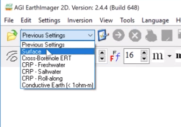
2. Reset to Surface defaults to avoid any previous settings (see image below) (Tip: Make sure on each start up of EarthImager™, that you reset to Surface defaults—especially if you're sharing EarthImager™ with others). Previous Settings are suitable if you do not close your session.
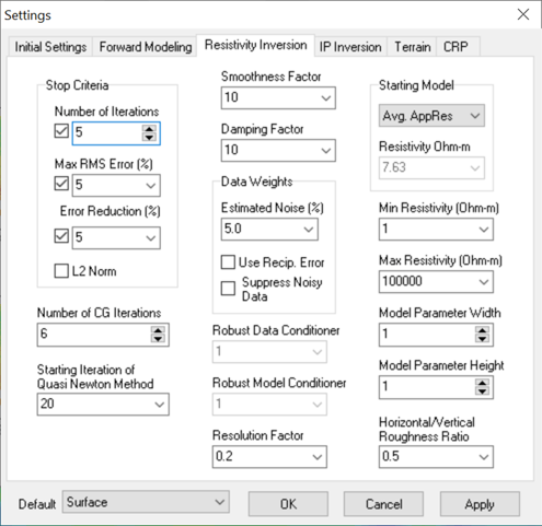
3. Most Surface data sets will have a little more noise than the Default Surface Settings. To minimize the chance of fitting to noise, it is best to make the following adjustments using Settings > Resistivity Inversion tab (see image) to adjust Stop Criteria > Number of Iterations = 5 and Data Weights > Estimated Noise = 5%
4. Now Load your STG file (raw data) using File > Read Data or the yellow folder icon with green arrow in the top left of the tool bar
5. Now is a good time to check data quality regarding signal levels and noise.
Select Edit > Data Editing Statistics
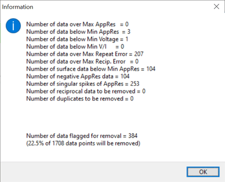
The Data Editing Statistics above are from a site where the operators positioned a line over and near several metal grates in an industrial site. The initial filters will remove an alarming amount of data. The resulting models would not converge to a good solution after several histogram data removal filters. Avoid removing more than 30% of the total data by the time you finish inversion models while using the over sampled AGI dipole-dipole command file or the optimal AGI dipole-dipole + strong gradient. Additional help on command files and line layout is here at the AGI Help Desk
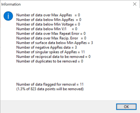
The Data Editing Statistics above are from a site where the operators made sure contact resistances were low and the line layout was good regarding buried metallic infrastructure.
4. You can turn on Remove Spikes by going to Settings > Initial Settings tab (see image below). (Note: A spike would typically exhibit itself as a singular extreme apparent resistivity value such as when the highest and lowest values are right next to each other in the raw data. These spikes will eventually filter out, but it is helpful for most data to remove them up front.)
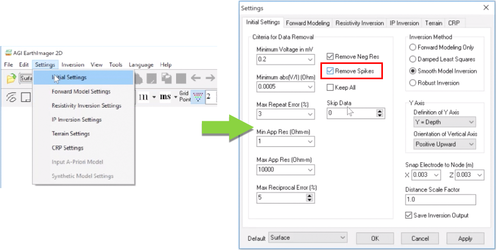
5. Leave all other settings the same as they are interrelated and changing them often causes artifacts
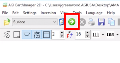
6. Run 1 model by pressing the green arrow button in the top left of the tool bar (see image below).
7. Right click on the inversion model (bottom most section) and select View Data Misfit Crossplot (see image below)
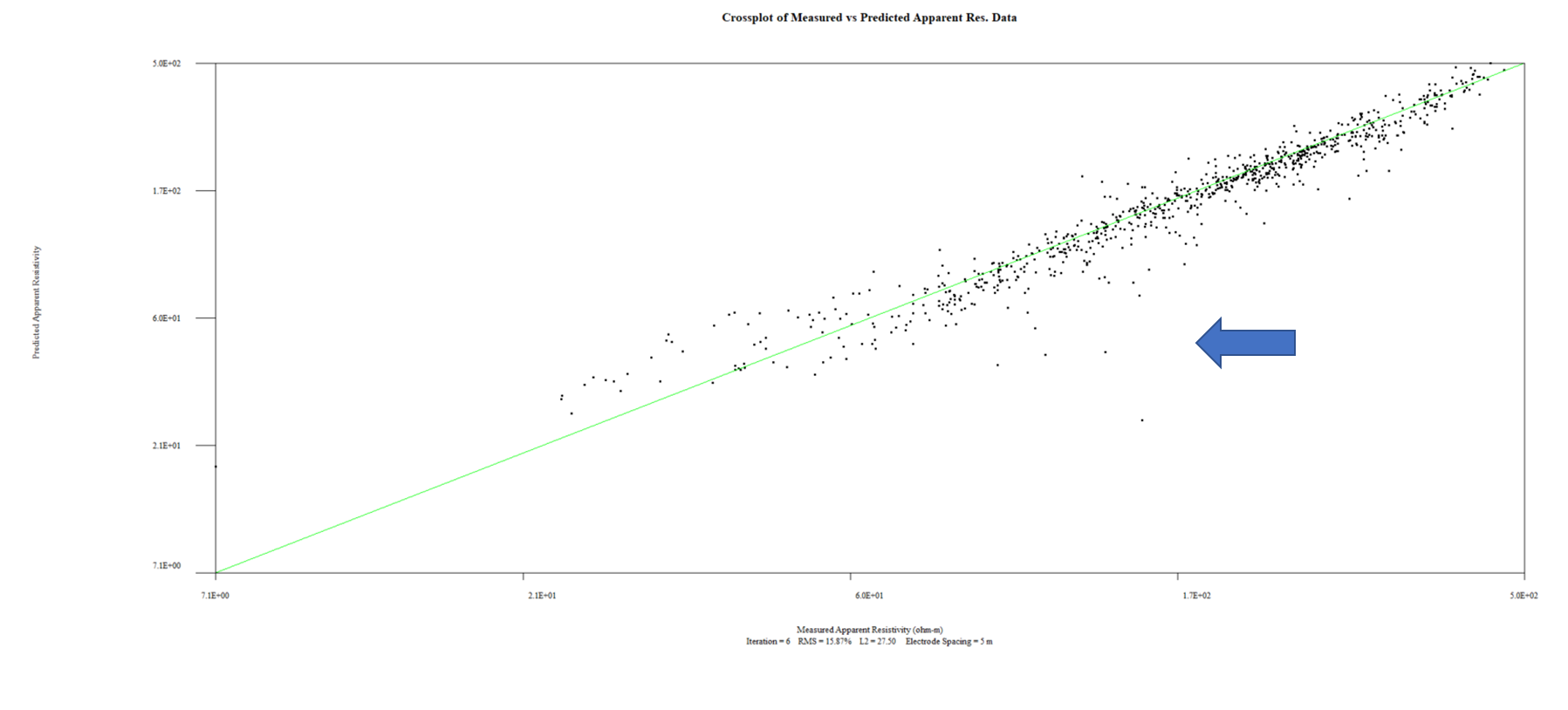
8. You will likely see several outliers from the 1:1 line showing raw predicted vs measured
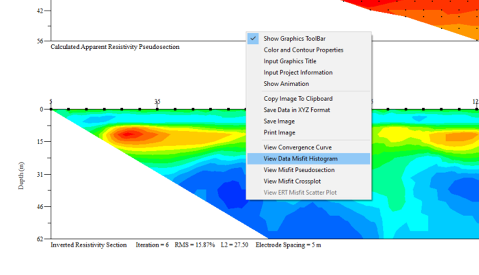
9. Right click again and select View Data Misfit Histogram data removal filter
10. Move the blue line left and right using the arrow keys on your keyboard. Keep your eye on the bottom of the window where Number of Data Removed = X is shown (see image below). Move the blue line to a point where X is ≤5%.
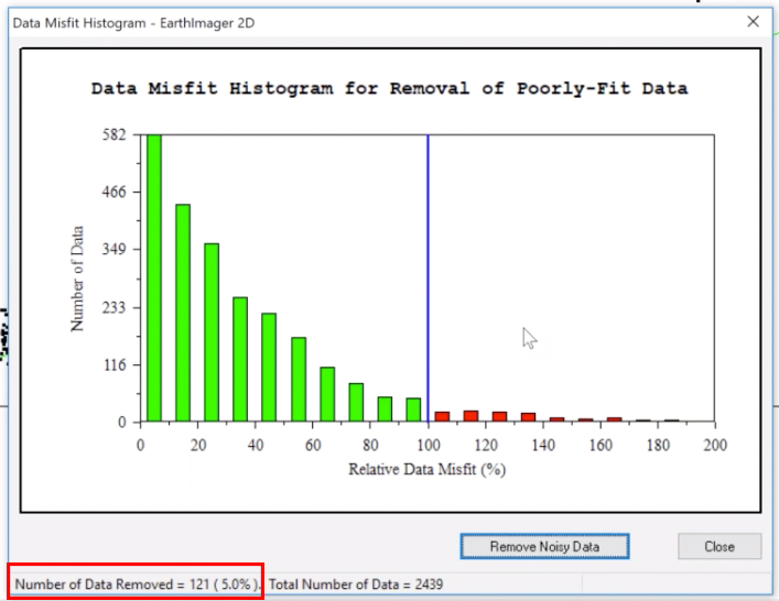
11. Click Remove Noisy Data button and the tool will then close
12. Run the model again by clicking the green arrow in the tool bar up top
13. Repeat this process until you see a tight fit on the cross plot and/or reasonable RMS compared to the first model. (For example, if your first model converged to 50% RMS, you will likely want to stop at ≤10% RMS for the final model. Very clean data is typically 5% or less.)
14. Save a JPEG of the cross plot
15. Save the Raw, Forward, and Inverted Resistivity Plot
16. In the main menu, go to View > Inverted Resistivity Section
17. Change Aspect Ratio to 1.0 unless you have space constraints. A drop down bow is in the middle of the tool bar
18. Keep color contours to the range shown that are unique to each line. It is common to have wide ranges in resistivity from line to line so a fixed or normalized color scale will obscure the structure.
19. Select the clip boundaries button (A small triangle symbol is over this button in the tool bar).
20. Use 1.0 as the aspect ratio unless you have steep topography included
21. Save the inverted model by right clicking and selecting file type